What did I learn from Advance Regression Project?
Github: Advance House Regression Techniques

In this blog I will try to give my experience of what I learned from the kaggle competition, Boston House Prediction where we have to build Machine learning model that will predict the house price based on several factors. These factors can be YearBuilt, YearRemodeled, SquareFoot, Basement etc. All these data was given in comma-seperated-values(csv) format.
Data Processing
This part is the most crucial step in creating any Machine Learning or Data Science in general. This step is called as Data Preprocessing. Data Scientist around world spends more than 60% of their time understanding and cleaning the data. Always remember clean data with weak model will outperform raw data and powerful model.
1. Check the data types of the columns.
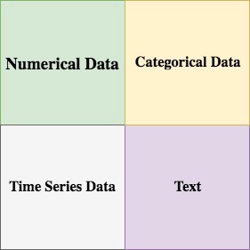
First thing I did was check datatypes of all columns. This will give me good view of what I am dealing with. There are several types of datatypes but these 4 are important.

Here’s an awesome blog explaining datatypes from machine learning perspective!
2. Fix the datatypes.
Now that I have looked at datatypes of the column using my own experience and some analysis later I fixed some datatypes that were wrongly configured.
3. Correlation Matrix
Correlation matrix put simply is used to look at the relationship between the variables. This blog will give you thorough knowledge on correlation matrix.
4. Check for the null values in the dataset.
After some more analysis it was time for checking null values. Null values can easily hurt the performance of our model. Null values are represented in different format like ‘?’ or ‘NAN’ or ‘_’
5. Fill the null values with appropiate values.
To deal with null values I used pandas libraries and replace the null values with median, mode and mean as required. Most of the numeric values were replaced by mean.
6. Visualize our target value ie. SalePrice.
After some clean up we can visualize our Target variable so I used ‘Seaborn’s’ library to visualize distribution of the target. What I saw shook me to the core 😂. I saw that target value was not normally distributed it was right skewed.
7. Normalize our target value.
Since our target variable was not normally distributed we can easily use np.log function from numpy to normally distribute our target column. High skewed variable could also cost some performance to our model. And for regression , it is convenient to transform highly skewed variables into a more normalized dataset.
8. Outlier Detection.
Now was time to detect some special variables which can be create huge impact on our model (negatively). These variables are called outliers. These variables can easily be detect with the help of visualization. I used boxplot and scatter plot to get these outliers.
9. Removing outliers.
Removing outliers are easy if you have good knowledge of pandas libraries. We just want to remove the variable that is farthest from our mean. MachineLearningMastery has a good blog that explains outlier removal technquies.
10. Drop Unwanted Columns
Since we are on topic of removal lets remove some unwanted columns that are of no use to our Machine learning model. For ex. (Id of the house), (House name), etc.
- Remember: For machine learning model to not overfit to our data we want as much data/column so removing columns not always a great choice.
11. Create Features/Columns
Creating more columns can benefit our ML model. So I created some columns like total space ie. (Basement + 1stFloor + SecondFloor). Creating feature comes after some experience or after thorough research in that field.
12. Normality Test.
Normality tests are used to determine if a data set is well-modeled by a normal distribution and to compute how likely it is for a random variable underlying the data set to be normally distributed. Source: Wikipedia
13. Box-Cox Transformation.
Box-Cox Transformation is used just like np.log but we convert non-normal dependent variable into normal. This is a good way of creating Normal Distribution on dependent variables.
14. Robust Scalar values.
Unscaled data can also slow down or even prevent the convergence of the gradient. Robust Scalar is use to scale the data between 0-1 and takes cares of the outliers. AwesomeBlog on Scaling Values with visualization
15. OneHotEncoding our columns.
OneHot Encoding is use to convert categorical variables to numerical values.
Example:
| Cat | Dog | Rabbit |
|---|---|---|
| 1 | 0 | 0 |
| 0 | 1 | 0 |
| 0 | 0 | 1 |
16. Setting up K-Fold CrossValidation
K-fold is use to check our model’s skill. K-fold is easy to implement and easy to use.
The general procedure is as follows:
- Shuffle the dataset randomly.
- Split the dataset into k groups.
- For each unique group:
Take the group as a hold out or test data set
Take the remaining groups as a training data set
Fit a model on the training set and evaluate it on the test set
Retain the evaluation score and discard the model
Summarize the skill of the model using the sample of model evaluation scores
Pheww!! Data cleaning is done, after suffering comes Happiness
Model Selection
I will not explain all the model’s here for that I think I will write another blog.
Here are all the models that I used for creating Dragon Model(Stacked Model)
- Lasso Regression Model
- Ridge Regression Model
- ElasticNet Regression Model
- GradinetBoosting Regressor Model
- Random Forest Regressor Model
- Support Vector Regressor (SVR)
- Xtreme Gradient Boosting (XGB)
- Light Gradient Boosting Model (LGBM)
One thing I want to shed some light on is Hyperparameter Tuning. I used Grid search. Grid search is arguably the most basic hyperparameter tuning method. With this technique, we simply build a model for each possible combination of all of the hyperparameter values provided, evaluating each model, and selecting the architecture which produces the best results.
For example, in Lasso Regression we would define list of values to try for alpha and grid search will build the model for all possible combination.
#preset alpha's value
alphas = [5e-05, 0.0001, 0.0002, 0.0003, 0.0004, 0.0005, 0.0006, 0.0007, 0.0008, 0.0009]
# calling Lasso function from sklearn
lasso = Lasso()
# using GridSearchCV to create all possible combinations
# lasso_search will get the best possible combination
# cv=kfold -> what we initialized at during data preprocessing phase
# scoring method is negative mean squared error this return the negated value of the metric.
lasso_search = GridSearchCV(lasso, {'alpha' : alphas} , cv=kfold, scoring="neg_mean_squared_error")
# fit function is use to fit the variables to the lasso_search.
lasso_search.fit(X, y)
# here we will print the best_estimators of lasso
lasso_search.best_estimator_
----------------------------------------------------------------------------
OUTPUT:
Lasso(alpha=0.0002, copy_X=True, fit_intercept=True, max_iter=1000,
      normalize=False, positive=False, precompute=False, random_state=None,
      selection='cyclic', tol=0.0001, warm_start=False)
Now we got the best possible combination for Lasso Regression on dataset. Time to make pipeline and score it against our evaluation metric ie. root mean squared error
# define our evaluation metric
def rmse_cv(model):
    mse = np.sqrt(-cross_val_score(model, X, y, scoring="neg_mean_squared_error" ,cv=kfolds))
    print(f'{model.__class__.__name__} score : {mse.mean():.4f}, {mse.std():.4f}')

# creating pipeline using sklearn is supersimple
# robustscalar to remove outliers and scale our data
# lasso values that we got from the above code.
lasso_model = make_pipeline(RobustScaler(),
                            Lasso(alpha=0.0002, random_state=2020)
                           )
# evaluation of model
rmse_cv(lasso_model)
----------------------------------------------------------------------------
OUTPUT:
Pipeline score : 0.1032, 0.0060
Now do this for all the model listed above.
Dragon Model
Dragon model consist of all the models listed above. Sklearn make’s it super easy to combine these models and create a new more optimized model. GeneralizationStacking also know as Blending is used when we have to create a more robust model using other models as base model.
I used XGB model as base or meta_regressor.
n_jobs= -1 is used to use all core of the cpu for model training.
| Model Name | Mean Score | Mean Std |
|---|---|---|
| Lasso | 0.1032 | 0.0060 |
| Ridge | 0.1032 | 0.0060 |
| Elastic | 0.1036 | 0.0065 |
| GradientBoostingRegressor | 0.1146 | 0.0052 |
| RandomForestRegressor | 0.1038 | 0.0069 |
| LGBMRegressor | 0.1123 | 0.0086 |
All the score’s I got from all the models.
Note: These are all pipeline scores that we fit our dataset to.
# all the models listed here
estimators = [lasso_model, ridge_model, elastic_model, gbR_model , rf_model,
              svr_model, xgb_model, lgbm_model]
# using StackingCVRegressor function avaliable in sklearn
stack_model = StackingCVRegressor(estimators,
                                  meta_regressor=xgb_model,
                                  n_jobs=-1,
                                  use_features_in_secondary=True)
# evaluation our dragon model
rmse_cv(stack_model)
----------------------------------------------------------------------------
OUTPUT:
StackingCVRegressor score : 0.1089, 0.0060
Lets check our Root mean square log error (RMSLE) score.
We will crosscheck our target values with the predicted values from the model using RMSLE
::: Individual Scores :::
| Model Name | RMSLE Score |
|---|---|
| Lasso | 0.08626 |
| Ridge | 0.087937 |
| Elastic | 0.087803 |
| GBR Model | 0.066912 |
| RandomForestRegressor | 0.076230 |
| SupportVectorRegressor | 0.081457 |
| XGB | 0.049099 |
| LGBM | 0.079329 |
| Stacked Model | 0.0487376 |